Code that I often use but rarely recall

Specifically, these snippets enable me to:

1. Customise quarto output

2. Generate ggplot2 charts in the style that I use

3. Format tables in my preferred way

4. Access databases inside and outside of shiny

5. Solve common niggles in package building

To demonstrate these code snippets, I’ll use the tidyverse packages with data from palmerpenguins.

suppressPackageStartupMessages(library(tidyverse))
library(palmerpenguins)

Note: In each case below, you can copy the code by hovering over it and selecting the clipboard icon in the top-right of the code chunk.

1. Customise quarto output

Given my frequent use of Quarto notebooks, I’ve gravitated to these settings that work best for me.

However, you can easily tweak these settings to suit you, as each option has an accompanying ‘tab auto-complete’ feature.

---
title: "Add title here"
subtitle: "Add subtitle here"
author:
  - Robin Penfold 
date: today
format: 
  html:
    anchor-sections: true 
    code-copy: hover 
    code-fold: true 
    code-link: true 
    code-overflow: wrap 
    code-summary: "</>" 
    code-tools: false 
    df-print: paged 
    embed-resources: true 
    float: true
    footnotes-hover: true 
    highlight-style: pygments
    lang: en-GB 
    linkcolor: "#63431c"
    mainfont: "Arial"
    table-of-contents: true 
    toc-depth: 4
    toc-title: " "
    title-block-banner: "#edd9c0"
    title-block-banner-color: "#63431c"
    title-block-categories: false
editor_options:
  chunk_output_type: inline
---

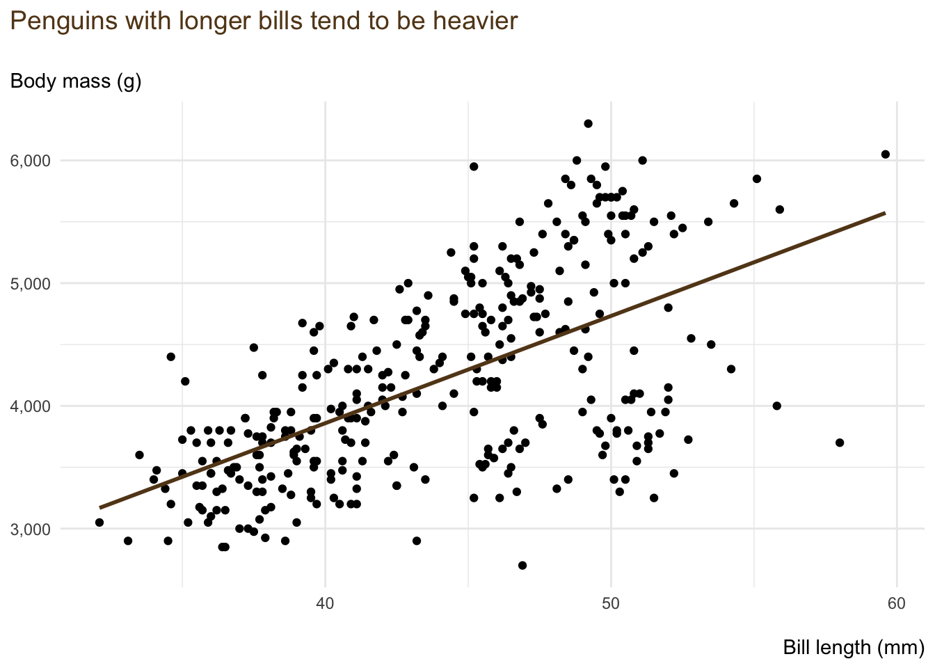
2. Generate ggplot2 charts in the style that I use

Over time, I have coalesced towards the following small chunk of code that builds (what I consider to be) a decent-looking chart in ggplot2.

penguins |> 
  ggplot(
    aes(
      x = bill_length_mm,
      y = body_mass_g
      )
    ) + 
  geom_point() +
  geom_smooth(
    method = "lm", 
    se = FALSE, 
    colour = "#63431c"
    ) +
  labs(
    title = "Penguins with longer bills tend to be heavier\n",
    subtitle = "Body mass (g)",
    x = "\nBill length (mm)",
    y = NULL
    ) +
  scale_y_continuous(labels = scales::label_comma()) +
  theme_minimal() +
  theme(
    plot.title.position = "plot",
    plot.title = element_text(size = 14, colour = "#63431c"),
    axis.title.x = element_text(hjust = 1)
    )

3. Format tables in my preferred way

I occasionally print tables using the out-of-the-box settings (admittedly tweaked by using the df-print: paged option in part 1 above). This generates a table as follows.

penguins

Otherwise, I usually use reactable with the following tweaks.

library(reactable)

penguins |> 
  select(species, island, bill_length_mm, bill_depth_mm, body_mass_g) |> 
  reactable(
    filterable = TRUE, 
    highlight = TRUE, 
    borderless = TRUE, 
    defaultPageSize = 5, 
    columns = list(
      species = colDef(name = "Species", minWidth = 90, sticky = "left"),
      island = colDef(name = "Island", minWidth = 90, sticky = "left"),
      bill_length_mm = colDef(name = "Bill length", sticky = "right", filterable = FALSE, format = colFormat(separators = TRUE, digits = 1)),
      bill_depth_mm = colDef(name = "Bill depth", sticky = "right", filterable = FALSE, format = colFormat(separators = TRUE, digits = 1)),
      body_mass_g = colDef(name = "Body mass", sticky = "right", filterable = FALSE, format = colFormat(separators = TRUE, digits = 0))
      )
    )

For completeness, I occasionally also use DT (i.e. the datatable package).

library(DT)

penguins |> 
  select("Species" = species, "Island" = island, "Bill length" = bill_length_mm, "Bill depth" = bill_depth_mm, "Body mass" = body_mass_g) |> 
  datatable(
    rownames = FALSE, 
    width = "100%",
    options=list(
      dom = 'tip',
      pageLength = 5
      )
    ) |> 
  formatRound(
    columns = 3:4,
    digits = 1
    ) |> 
  formatRound(
    columns = 5,
    digits = 0
    )

4. Access databases inside and outside of shiny

I use the wonderful DBI and dbplyr all the time, not least for exploratory analysis.

(Note that whilst I typically don’t use SQLite, I will do so here, as it plays better with my website architecture.)

library(RSQLite)

con <- dbConnect(RSQLite::SQLite(), ":memory:")

dbWriteTable(con, "instruments", dplyr::band_instruments)
dbWriteTable(con, "members", dplyr::band_members)

dbListTables(con)

[1] "instruments" "members"    

In this example, we create an object (con) for connecting to the SQLite database, where we add two tiny tables, called instruments and members. We can then explore these tables.

tbl(src = con, "instruments")

tbl(src = con, "members")

Even better, we can explore the tables when they are combined and tidied. (Whilst the code appears to return all the data, that’s only because our tables are uncommonly small.)

tbl(src = con, "instruments") |> 
  left_join(
    tbl(src = con, "members"), 
    by = "name"
  ) |> 
  filter(band == "Beatles")

Once you have what you need, assign a name to the code and append it with |> collect().

Whilst this functionality is great outside of shiny, it is often more valuable within it. (After all, these apps can be a really safe and simple way for users to access a corporate database.)

To do so, some other tweaks are required within shiny’s server functionality, as illustrated below.

data_chosen <- shiny::reactive({
  shiny::req(input$dataset)
  main_data |> 
    dplyr::filter(name_dataset == input$dataset) |> 
    dplyr::mutate(id = as.integer(id))
  })

data_chosen_id <- shiny::reactive(
  quote({data_chosen()$id}),
  quoted = TRUE
  )

data_calculated <- shiny::reactive({
  arbitrary_function(
    con,
    arbitrary_argument = data_chosen_id()
    )
  })

5. Solve common niggles in package building

When I’m building packages, I often get dinged with notes or warnings about two common package niggles.

The first of these is non-ASCII characters. With apologies for the person who showed me, and who I now can’t recall, you can find these characters by:

• Clicking CTRL + F in RStudio

• Selecting the Regex tick-box

• Entering: [\u0080-\uFFFF] or [^\x00-\x7F] as the search term

From there, you can use stringi::stri_escape_unicode('@') to get the Unicode equivalent for @. (Note that you also might need to remove the initial ‘\’ on Windows.)

The second niggle of package building concerns variable binding. It occurs during the package check and creates a note along the following lines.

no visible binding for global variable
    ‘ABC’

In this case, we need to do something of the form below (from my simple package p0bservations that you can find here).

#' @title Calculate income net of UK tax and National Insurance
#'
#' @description This function ...
#' @param income_taxable The taxable income level ...
#' @param tax_year_end The calendar year in which the tax year ends ...
#' @export
#' @examples
#' \dontrun{
#' calc_income_net(income_taxable = 38000, tax_year_end = 2022L)
#' }
#' 
#' @importFrom rlang .data

Once we have added the line of #' @importFrom rlang .data, we can call the variables as follows (i.e. as before, but preceded by .data$).

year_tax_end_options <- p0bservations::tax_parameters |> 
  dplyr::distinct(.data$year_tax_end) |> 
  dplyr::pull(.data$year_tax_end)

Once again, I hope that this aide-mémoire helps you as well as me!