Brexit vote analysis

You can scroll down for an interactive chart of each constituency, but the following chart shows the main detail.

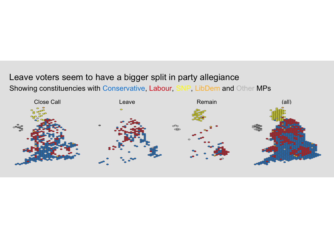
library(dplyr)
library(forcats)
library(ggiraph)
library(glue)
library(ggplot2)
library(ggtext)
library(parlitools)
library(scales)

map_details <- west_hex_map
sf::st_crs(map_details) = 4326

data_brexit <- leave_votes_west |>  
  rename(`Leave Vote` = figure_to_use) |> 
  mutate(
    `Party of MP` = as_factor(party_2016), 
    `Party of MP` = 
      recode(
        `Party of MP`,
        `Scottish National Party` = "SNP", 
        `Liberal Democrat` = "LibDem"
        ),
    `Party of MP` = fct_lump(
      `Party of MP`,
      n = 5, 
      other_level = "Other"
      )
    ) |> 
  left_join(
    map_details,
    by = c("ons_const_id" = "gss_code")
    ) |> 
  mutate(
    constituency = if_else(
      is.na(constituency_name.x), 
      constituency_name.y, 
      constituency_name.x
      ),
    vote_status = case_when(
      (`Leave Vote` >= 0) & (`Leave Vote` <= 0.4) ~ "Remain",
      (`Leave Vote` > 0.4) & (`Leave Vote` <= 0.6) ~ "Close Call",
      (`Leave Vote` > 0.6) & (`Leave Vote` <= 1) ~ "Leave",
      TRUE ~ "Error"
      ),
    vote_status = as_factor(vote_status),
    vote_status = fct_relevel(vote_status, sort)
    ) |> 
  select(constituency, `Leave Vote`, `Party of MP`, ons_const_id, vote_status, geometry)

html_text <- glue("<span>Showing constituencies with <span style='color:#0087DC;'>Conservative</span>, <span style='color:#DC241F;'>Labour</span>, <span style='color:#FFFF00;'>SNP</span>, <span style='color:#FDBB30;'>LibDem</span> and <span style='color:#AFAFAFAF;'>Other</span> MPs</span><br/>")

data_brexit |> 
  ggplot() + 
  geom_sf(
    aes(
      group = constituency,
      geometry = geometry,
      fill = `Party of MP`
      ),
    size = 0.1
    ) + 
  scale_fill_manual(
    values = c(
      Conservative = "#0087DC",
      Labour = "#DC241F",
      SNP = "#FFFF00",
      LibDem = "#FDBB30",
      Other = "grey80"
      )
    ) + 
  facet_grid(~vote_status, margins = TRUE, drop = TRUE) +
  theme_void() + 
  labs(
    title = "Leave voters seem to have a bigger split in party allegiance",
    subtitle = html_text
  ) + 
  theme(
    plot.title.position = "plot",
    plot.subtitle = element_markdown(),
    legend.position = "none",
    plot.background = element_rect(
      fill = "grey90", 
      colour = "grey90", 
      linewidth = 1
      ),
    plot.margin = margin(0.5, 0.5, 0.5, 0.5, "cm")
    )

Basically, outside of Scotland, there seems to be a bigger split in Leaver constituencies than in their Remainer counterparts.

To get the details for each constituency, hover over the relevant spot in the chart below.

gg <- data_brexit |> 
  ggplot() + 
  geom_sf_interactive(
    aes(
      group = constituency,
      geometry = geometry,
      fill = `Leave Vote`,
      colour = `Party of MP`,
      tooltip = paste0(
        constituency, 
        "\n MP: ",
        `Party of MP`,
        "\n Leave vote: ",
        round(`Leave Vote` * 100, 0),
        "%"
        )
    ),
    size = 0.1
  ) + 
  scale_fill_gradient_interactive(
    low = "white", 
    high = "#63666a",
    labels = percent_format(accuracy = 1)
    ) +
  scale_colour_manual_interactive(
    values = c(
      Conservative = "#0087DC",
      Labour = "#DC241F",
      SNP = "#FFFF00",
      LibDem = "#FDBB30",
      Other = "grey80"
      )
    ) + 
  theme_void() +
  labs(
    title = "Leave vote and winning party, by constituency", 
    subtitle = "Hover over a point for the details"
  ) + 
  theme(
    legend.position = "right",
    legend.text = element_text(size = 6, hjust = 0),
    legend.title = element_text(size = 8)
    )

girafe(ggobj = gg)